
Merkle Trees
Important note: When I started this blog, I promised myself I wouldn’t overuse mathematical concepts or notation. But what you can resist—and what you can’t—is carved in your blood. So here we are. And sure, I could pretend this is justified because “hey guys, we’re talking crypto—how else would you do it without Math?”
But the truth is much simpler. Whenever I start doing math, a voice in my sadistic mind begins to yell: “I love math — it makes people cry.”
Preliminary apologies: The math rendering is courtesy of my ongoing feud with Jekyll. If the formulas look like crap, that’s a feature showing authenticity.
Definition 1
The syntax \(\{0,1\}^*\) denotes the set of strings built on the alphabet \(\{0,1\}\) of arbitrary length.
In other words, the following relations hold true:
- \(001000110100\in\{0,1\}^*\)
- \(0\in\{0,1\}^*\)
- \(010101\dots 0101010101\in\{0,1\}^*\)
Observe that if \(\varepsilon\) denotes the empty string, then also \(\varepsilon\in\{0,1\}^*\)
Observation 1
For all \(k\in\mathbb{N}\), the set \(\{0,1\}^k\) is the set of all the strings over the alphabet \(\{0,1\}\) having length \(k\). All its elements are also elements of \(\{0,1\}^*\) , for a string of a given length also belongs to the set of strings of arbitrary length. Therefore a more formal definition of \(\{0,1\}^{\ast}\) is \[\{0,1\}^{\ast} := \bigcup\limits_{i=0}^{\infty} \{0,1\}^{i}\] where \(\{0,1\}^0=\varepsilon\), the empty string.
Definition 2: Concatenation operator
Let \(k,h\in\mathbb{N}\), and let \(\kappa\in\{0,1\}^k\) and \(\eta\in\{0,1\}^h\). The concatenation of \(\kappa\) and \(\eta\) is the unique element of \(\{0,1\}^{k+h}\) whose first \(k\) bits coincide with those of \(\kappa\), and whose last \(h\) bits coincide with those of \(\eta\).
In general we define the concatenation operator as: \[\|:\{0,1\}^{\ast}\times\{0,1\}^{\ast}\rightarrow\{0,1\}^{\ast}\] An example may help clarify the concept. Let \(\kappa=10111\) and \(\eta=00100\). Then their concatenation is: \(\kappa\|\eta=1011100100\).
Definition 3: Cryptographic hash function
Let \(k \in \mathbb{N}\). A cryptographic hash function is a function \[H : \{0,1\}^* \rightarrow \{0,1\}^k\] mapping binary strings of arbitrary length to binary strings of fixed length \(k\).
The function H must satisfy the following security properties:
- Pre-image resistance Given \(y \in \{0,1\}^k\), it is computationally infeasible to find any \(x \in \{0,1\}^*\) such that \(H(x) = y\).
- Second pre-image resistance Given \(x \in \{0,1\}^{\ast}\), it is computationally infeasible to find a different \(x^{\prime} \in \{0,1\}^{\ast}\) with \(x^{\prime} \neq x\) such that \(H(x^{\prime}) = H(x)\).
- Collision resistance It is computationally infeasible to find any pair \(x, x’ \in \{0,1\}^*\) with \(x \neq x’\) such that \(H(x) = H(x’)\).
Observation 2
From now on, unless explicitly stated otherwise, we will denote by \(H\) a cryptographic hash function: \(H : \{0,1\}^* \rightarrow \{0,1\}^k\) and with \(d\) an element of \(\{0,1\}^{\ast}\). In this context, \(d\) stands for data, and it’s an arbitrary binary string.
We define the following operations.
Definition 4: Leaf tagging function
We define the leaf tagging function as: \[\operatorname{Leaf}(d):= H\bigl(0x00\|d\bigr)\] where the constant byte \(0x00\) is used to mark the input domain corresponding to tagged leaves.
Definition 5: Internal node tagging function
Let \(x\) and \(y\) be two elements of \(\{0,1\}^k\). We define the internal node tagging function as: \[\operatorname{Node}(x,y):= H\bigl(0x01\|x\|y\bigr)\] where the constant byte \(0x01\) is used to mark the input domain corresponding to internal nodes.
Observation 3
By abuse of notation, when no confusion arises we may write \(\operatorname{Node}(x,y)\) as \(H(0x01 \,\|\, x \,\|\, y)\) and \(\operatorname{Leaf}(d)\) as \(H(0x00 \,\|\, d)\), omitting explicit mention of the tagging convention.
Perhaps the underlying idea is already taking shape in your mind, but let’s enrich this theory with:
Definition 6: Tagged tree
A tagged hash tree is a binary tree where:
- each leaf stores a value of the form \(\operatorname{Leaf}(d)\);
- each internal node stores a value of the form \(\operatorname{Node}(x,y)\);
- the root is the recursively defined tag-propagated hash.
Now we can formalise the following:
Definition 7: Merkle tree
A Merkle tree is a particular instance of a tagged hash tree obtained by recursively applying the leaf and internal-node tagging functions defined above. More precisely:
- Each leaf of the tree corresponds to a data block \(d \in \{0,1\}^*\) and stores the value \(\operatorname{Leaf}(d) = H(0x00 \,\|\, d)\).
- Each internal node with left child \(x\) and right child \(y\), both belonging to \(\{0,1\}^k\), stores the value \(\operatorname{Node}(x,y) = H(0x01 \,\|\, x \,\|\, y)\).
- The Merkle root is the value stored at the root of the tree, obtained by recursively propagating the tagged hashes from the leaves to the top.
In other words, a Merkle tree is a tagged hash tree whose structure is entirely determined by the recursive application of the \(\operatorname{Leaf}\) and \(\operatorname{Node}\) functions, and whose root provides a cryptographic commitment to all the underlying data blocks.
Definition 8: Merkle proof
Let \(T\) be a Merkle tree with leaves associated to data blocks \(d_0, d_1, \dots, d_{n-1} \in \{0,1\}^*\), and let \(d_i\) be one such block.
Let \(L_i := \operatorname{Leaf}(d_i)\) denote the value stored at the corresponding leaf.
Let the depth of the tree be \(p\), so that the root lies at level \(p\).
A Merkle proof for \(d_i\) with respect to the root \(R\) is a finite sequence \[\pi_i = \bigl((h_0, b_0), (h_1, b_1), \dots, (h_{p-1}, b_{p-1})\bigr)\] Given \(L_i\), define the sequence \(x_0, x_1, \dots, x_p\) recursively by \[x_0 := L_i\] and, for each \(j \in \{0,\dots,p-1\}\), \[x_{j+1} := \begin{cases} \operatorname{Node}(h_j, x_j) = H(0x01 \,\|\, h_j \,\|\, x_j), & \text{if } b_j = L, \\[6pt] \operatorname{Node}(x_j, h_j) = H(0x01 \,\|\, x_j \,\|\, h_j), & \text{if } b_j = R. \end{cases}\]
The sequence \(\pi_i\) is a valid Merkle proof for \(d_i\) (with respect to \(R\)) if and only if \(x_p = R\).
In other words, a Merkle proof for \(d_i\) is precisely the information needed to reconstruct the root value \(R\) from \(L_i\) by successively combining it with its sibling nodes in the correct left/right order.
Proposition 1: Integrity propagation
Let \(T\) be a Merkle tree with root value \(R\).
Assume that the hash function \(H : \{0,1\}^* \rightarrow \{0,1\}^k\) is collision-resistant.
Then any modification of a data block \(d_i\) at the leaves changes the value of the Merkle root with overwhelming probability.
Proof (sketch)
Let \(d_i’\neq d_i\) be a modification of the data block \(d_i\). By Definition 4, the leaf values are \[\operatorname{Leaf}(d_i) = H(0x00 \,\|\, d_i), \qquad \operatorname{Leaf}(d_i’) = H(0x00 \,\|\, d_i’)\] If these two values were equal, i.e. \(H(0x00 \,\|\, d_i) = H(0x00 \,\|\, d_i’)\), then \((0x00 \,\|\, d_i)\) and \((0x00 \,\|\, d_i’)\) would form a collision for \(H\), contradicting collision resistance. Hence: \(\operatorname{Leaf}(d_i) \neq \operatorname{Leaf}(d_i’)\).
By Definition 5, every internal node value is obtained by applying \(\operatorname{Node}(x,y) = H(0x01 \,\|\, x \,\|\, y)\), so any change in a child value forces a change in its parent value unless a collision is found in \(H\). Therefore the change in the leaf propagates to all its ancestors.
Since the root is an ancestor of every leaf, its value must also change unless a collision occurs.
Under the collision-resistance assumption, this event has negligible probability.
Example 1: the construction of a Merkle tree
The following picture shows how a Merkle tree is constructed, from the leaf layer up to the root of the tree.
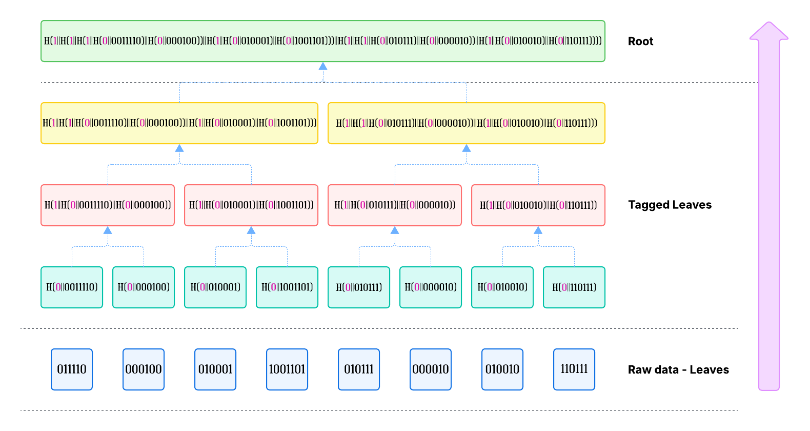
Hopefully, I did not make any mistakes while copy-pasting the strings. Apologies if I did.
Consider that the only variable elements, here, are the leaves. If the structure is properly segregated, the attack surface is limited to the set of leaves. Observe that also the order of the leaves is preserved in this structure - it’s enough to note that, for all strings \(a,b\in\{0,1\}^*\) , with \(a\neq b\), and for all cryptographic hash functions \(H\), we have \(H\bigl(a\|b\bigr)\neq H\bigl(b\|a\bigr)\) .
This means that swapping left and right children produces a completely different internal hash, and therefore a completely different root.
This simple property forces the Merkle root to encode not only what the data is, but also where each piece of data lies in the sequence. And this is exactly why Merkle trees are used in systems where order is a first-class security property:
- in blockchains, to guarantee the exact ordering of transactions;
- in code-signature chains, to ensure that signing steps cannot be reordered or interposed;
- in any structure where permutation of the input would constitute an attack vector.
The Merkle root is therefore a commitment not to “some set of values”, but to this precise ordered list of values. If you change the order of even two adjacent leaves, the root changes.
If you try to forge a leaf and keep the same root, you must break the collision resistance of H. Good luck with that.
The objection here could be that I used a set of data whose cardinality is an integer power of 2. True. I cheated, I admit. I cheated on purpose. The question now becomes what happens if the cardinality of the dataset is not a power of two? After all, this is the most frequent case in real cases (blockchains, distributed systems, storage, certificates, notarisation, and so on).
The standard solution is called Padding by duplication. This method is required in Ethereum, Bitcoin, Certificate transparency. Pretty much everywhere.
Example 2: Padding by duplication
We use an example to illustrate this technique.
Suppose we have five different leaves \(d_0, d_1, d_2, d_3, d_4\).
We need an even number of leaves to apply the previously described merge-and-hash algorithm, so a new leaf is introduced, obtained by duplication. The set becomes: \(d_0, d_1, d_2, d_3, d_4, d_5\) where \(d_5=d_4\).
Now the algorithm can be applied to obtain the values \(N_{1,0}=\operatorname{Node}(d_0, d_1), N_{1,1}=\operatorname{Node}(d_2, d_3)\) and \(N_{1,2}=\operatorname{Node}(d_4, d_5)\).
We now have three nodes, still an odd number - so we apply the rule again obtaining the nodes \(N_{1,0}, N_{1,1}, N_{1,2}, N_{1,3}\), where \(N_{1,3}=N_{1,2}\).
Now the cardinality of the dataset is even, and the algorithm can be applied. We obtain the values \(N_{2,0}=\operatorname{Node}(N_{1,0}, N_{1,1}), N_{2,1}=\operatorname{Node}(N_{1,2}, N_{1,3})\).
The cardinality of the dataset is even, and the algorithm can proceed (observe that the cardinality is an integer power of 2, so no further paddings will be required).
Next steps
- implementing the Data Type in our favourite language?
- implementing the Merkle tree operations?
- Build
- Proof generation
- Proof verification
- Update (leaf mutation)
- Root comparison
- Append (extension)
- Consistency proof
- Range proof
- Indexing
Want the deep dive?
If you’re a security researcher, incident responder, or part of a defensive team and you need the full technical details (labs, YARA sketches, telemetry tricks), email me at info@bytearchitect.io or DM me on X (@reveng3_org). I review legit requests personally and will share private analysis and artefacts to verified contacts only.
Prefer privacy-first contact? Tell me in the first message and I’ll share a PGP key.
Subscribe to The Byte Architect mailing list for release alerts and exclusive follow-ups.
Gabriel(e) Biondo
ByteArchitect · RevEng3 · Rusted Pieces · Sabbath Stones